Notes from September 29, 2000

The motivation for this particular class is to illustrate the source of common distributions. In Vining's book they seem to just fall from the sky onto our page. I wanted to illustrate how each is derived from another, and that they all build upon a few simple, but powerful ideas in probability.

• The binomial distribution is our most basic one. It results from counting successes in Bernoulli trials. We can derive it by applying the rules of probability that govern independent events. There are other discrete distributions that result from counting events in other circumstances, but the binomial is the most important one for our purposes.
• The Poisson distibution is the binomial distribution in the limit that the number of trials becomes infinite, and probability of success in each trial becomes infinitesimal, but their product remains a constant we can think of as the success rate.
• There are all sorts of ways to arrive at the normal distribution. I mentioned several in class. In addition to its importance in its own right, for our purposes today it was important to note that both the binomial and Poisson distributions tend to look like the normal distribution in the instance of large expected value, which means we can use the tabulated CDF of the normal distribution to evulated binomial and Poisson probabilities. For the binomial process this approximation requires np>5 or so depending on how close is p to a value of 1/2. For the Poisson distribution this requires alpha>5.
• When the probability of success per Bernoulli trial is extremely small, the normal approximation may be adequate for calculation, but the distribution will still have an obvious skew, which the Poisson distribution exhibits nicely.
• In most instances we know little about the distribution of our random variable (i.e. the parent population that our individuals come from), so we resort to sampling to learn about the population. This brings us to sampling distributions.
• Sampling distributions result from functions of random variables. As an example of a function of a random variable, I presented the Boltzmann distribution, which describes how energy is distributed among particles at thermal equilibrium, and the related Maxwell distribution of the speeds of the particle. These two distributions are related through the change of variable given by the formula for kinetic energy E=1/2mv².
• It is obvious that parameters which we derive from a random sample, which is but a subset of our population, will itself be a random variable. Successive samples drawn from the population will provide varying values of the parameter.
• We decided that the sum of samples drawn from a normal distribution would also be distributed normally, but that the variance would be larger than that of the parent population in proportion to the size of the sample.
• The mean value of a sample drawn from a normal distribution is an unbiased estimate of the mean of the parent population, but its variance is smaller in proportion to the size of the sample.
• It is very important that you recognize the following fact, which eludes so many beginning students of statistics. If a parent popluation is normally distributed, then the mean value of a random sample drawn from it is also normal. However, these are different distributions. One is the parent distribution, the other is the sample distribution. They have the same mean value, but different variance. The sample variance is always smaller, because the effect of a member of the sample with a value smaller than the parent mean is moderated, so to speak, by other sample members with values likely to be above the mean.
• We estimate population variance by summing together deviations of samples values from the mean of the sample. Such a statistic is obviously a random variable. Any random variable which is the sum of squared deviations of samples drawn from a normal population follows a distribution named Chi Squared.
• In most situations we know neither the true population mean nor the variance. We must estimate both through a sample. In order to assign confidence intervals to our statistics, and draw conclusions, we need a statistic that is the ratio of a normally distributed random variable, and the square root of one distributed as Chi Squared. This random variable follows a distribution named "Student's t." We call it the t statistic.
• Finally, in instances where we wish to compare two estimates of population variance, we require the distribution of a random variable that is the ratio of two random variables distributed as Chi Squared. Such a statistic is already available and is named Snedecor's F, or the Fisher statistic, or just F.

At this point I have introduced all of the discrete and continuous distributions that we use in this introductory class. Next class period we will work examples which show the utility of most of them. The rest will have to wait until we begin chapter 4 where we draw inferences from our statistics.

Notes from September 24, 1999

An example calculation of expected value of a function

Recall that E(y) = S yp(y) for a discrete RV and V(y)=E(y²)-[E(y)]²

E(Q)=E(g(y))=Sg(y)p(y)

Q(r)=CVo(1-e-ar).
E(Q) = SQ(r)p(r).

Example Problem
p=0.25  V=10volts  C=10e-6f   time constant=0.5sec
time step(n)    p       Q(n)      p(n)*Q(n)    p*Q(n)2    p(n)*n
       1        0.25 3.93469E-05 9.83673E-06 3.87045E-10       0.25
       2      0.1875 6.32121E-05 1.18523E-05 7.49206E-10      0.375
       3    0.140625 7.76870E-05 1.09247E-05 8.48709E-10   0.421875
       4  0.10546875 8.64665E-05 9.11951E-06 7.88532E-10   0.421875
       5 0.079101563 9.17915E-05 7.26085E-06 6.66484E-10 0.39550781
       6 0.059326172 9.50213E-05 5.63725E-06 5.35659E-10 0.35595703
       7 0.044494629 9.69803E-05 4.31510E-06 4.18480E-10 0.31146240
       8 0.033370972 9.81684E-05 3.27598E-06 3.21597E-10 0.26696777
       9 0.025028229 9.88891E-05 2.47502E-06 2.44752E-10 0.22525405
      10 0.018771172 9.93262E-05 1.86447E-06 1.85191E-10 0.18771171
      11 0.014078379 9.95913E-05 1.40208E-06 1.39635E-10 0.15486216
      12 0.010558784 9.97521E-05 1.05326E-06 1.05065E-10 0.12670540
Sums     0.968323648             6.90172E-05 5.39036E-09 3.49317836

E(Q)=   6.90172E-05Coulombs
V(Q)=   6.26976E-10
Std.Dev=2.50395E-05Coulombs

By comparison the calculation of E(Q) as E(n) substituted into the 
expression for Q(n) is 8.25632E-05 Coulomb which is 14% too high.

Back to the subject of extreme values.

We can write down the probability associated with a maximum value as follows.

P(X1=m,X2<=m,...,Xk<=m)=Probability of k items <=m.

P(X1=m,X2<=m,...,Xk<=m)=Cdf(m)*Cdf(m)*...*Cdf(m)

or, equivalently

P(X1=m,X2<=m,...,Xk<=m)=Cdf(m)k

Once again, this distribution is of the extreme value, and I mentioned that it is of great importance in engineering work. Now I will show you its importance. Often engineers design things to withstand unusual events. No doubt all of you have heard of the 100 year flood, or the 100 year wind gust, or whatever. Most people think of this as the greatest such event that will occur in 100 years, but this terminology leads people to think that such an event can happen only once in a hundred years. This is wrong thinking.

A better way to frame this is that the 100 year wind gust is an event that will happen once per 100 years on average if we examine a long enough historic record. In this sense the 100 year wind could occur in two successive years, but only on rare occasions. How rare is what we want to decide.

First, before we go very far into this discussion, I must provide one caveat. The distribution on which we base all this work assumes that samples of extreme whatever are independent samples. It is on this assumption that all our proud work may run aground. Obviously if we are examining wind gusts from day to day, then very windy days occur together. Thus the high wind gust on tuesday, for instance, is NOT independent of the gust on monday. They are correlated by the fact that storminess occurs over several days. Unfortunately this tendency occurs on longer time scales.

Beniot Mandelbrot showed that correlation, or lack of independence, occurs over the longest time scales imaginable in geophysical data. Windy days cluster together, as do windy years, and windy centuries and so forth. Mandelbrot has called this the "Joseph" effect for the prophet who foresaw lean years following years of plenty. Please keep in mind that geophysical data may not behave like random, independent samples, no matter how far apart in time they occur.

Second, also before we go too far, I need to define the return interval of an event. If an event has a probability of p of occuring during a sample interval, then it has a return interval T=1/p periods. For example, the odds of snake-eyes on the roll of two die is 1/36, so the return interval is 36 rolls. However, snake-eyes can turn up on two consecutive rolls.

One way to approach the problem of estimating probabilities and return periods is to simply look at whatever historical record one has, and estimate from the frequency of actual observations. There are two disadvantages in this. The most important is that it only provides an estimate of the greatest event so far observed. What of even larger events? Also, it leaves us to estimate using only a few events, maybe only one. We need a method for using all the available data, not just a few observed extremes.

The distribution of extreme values depends on the Cdf, which we can estimate very well using all our observed data. Then we make use of the distribution of the extreme Cdf(m)^k to extrapolate to events greater than any observed so far. So we have already derived all the tools we need to solve our problem. Let's look at real data to illustrate the method.

I have obtained daily temperature records for Portland for the period 1928-1996. The spreadsheet, which I have included on another web-page, shows the maximum temperatures recorded during the three summer months, June, July, and August. The record extreme temperature is 107F, and it occurred thrice in the 62 years of record. So the return interval of 107F temperature is roughly 21 years. Amazingly enough, these records occurred in 1941, 1964, and 1981; just about 20 years apart. This makes me terribly suspicious about long range correlation in the data, but we'll use it as an example just the same.

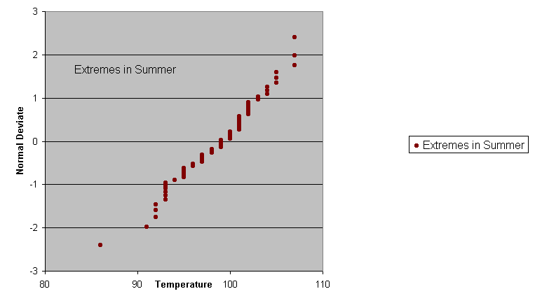
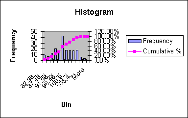
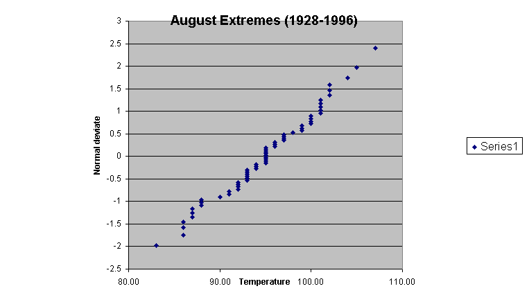
The next figures show probability plot of the data for the entire summer, and for the month of August. Vining would say that these plots show the data to be nearly normal, but I'm not so sure, especially after examining a histogram of the summers data.

Indeed, the histogram below shows that the distribution of extreme temperatures for each month (3 per each summer) follow a skewed distribution that is probably unimodal, but definitely not normal.