Kevin T. Kilty, March 1999
Teresa Imanishi-Kari was alleged to have falsified experiments, and data, in her laboratory notebooks. She was exonerated of all charges in 1996, but only after a Kafka-esque decade in which the charges against her continually metamorphosed, during which she could not actually examine the specific charges or evidence against her, and during which she was characterized as an example of corrupt science by government oversight committees. One of the principal charges against her was that she had cobbled together a laboratory notebook to bolster her claim of having performed experiments on immune response -- experiments which lead to an acclaimed paper in the journal Cell.
Imanishi-Kari's notebooks were apparently very messy and difficult to decipher. They contained paper strips of instrument readings that were taped to pages, and which were in varying colors and degrees of fadedness, printed with varying ribbons on a variety of printers. The pages themselves appeared out of order, dates were scratched through and corrected, there was white-out correction fluid used back-to-back on both sides of some sheets, and mechanical impressions suggested that pages were, in fact, dated out of the order they were written. The question naturally arose whether this messiness was the product of a clumsy, hurried attempt to deceive. Thus, the U. S. Secret Service was asked to perform forensic analysis on the notebooks. Part of the forensics was to compare Imanishi-Kari's notebooks against a sample of the notebooks of other scientists.
Secret Service investigators were unable to examine more than a tiny fraction (an estimate was perhaps 1%) of the notebooks produced by researchers in the same laboratory during the same time period. In the forum of the hearing, Imanishi-Kari's counsel cross examined one of the Secret Service investigators about why he had not included for examiniation the laboratory notebook of Moema Reis, at one time a research collaborator of Imanishi-Kari. The agent testified that they excluded this notebook because it looked a lot like that of Imanishi-Kari so they were "...unwilling to use that as an example of what a normal or a usual notebook would be."
Since an explicit goal of the comparison was to establish the normalcy of Imanishi-Kari's notebook, the decision to exclude other notebooks that looked like hers becomes an implicit definition of hers as being abnormal. The neat circular logic is...
There is no means of explaining the nature of this circular argument without referring extensively to an earlier study (Study #1) which explains in detail how a particular inverse method behaves. Then in a later study, the method is applied in a way that is circular.
The objective of this method is to use temperature measured in a borehole to figure what the ground surface temperature (GST) was like over the past 1000 years. To do this the authors make a model of temperatures in the subsurface, combined with a computer program that uses the observed temperatures to find the parameters of the model. The central idea is to begin with a initial set of parameters for the model, which I denote here symbolically as mo , and systematically adjust the parameters to minimize an objective function like the following...
S=misfit to observations + change from initial model
Or mathematically...
S=(d-do)tCd-1(d-do) +(m-mo)tCm-1(m-mo).
The reason for using this objective is as follows.
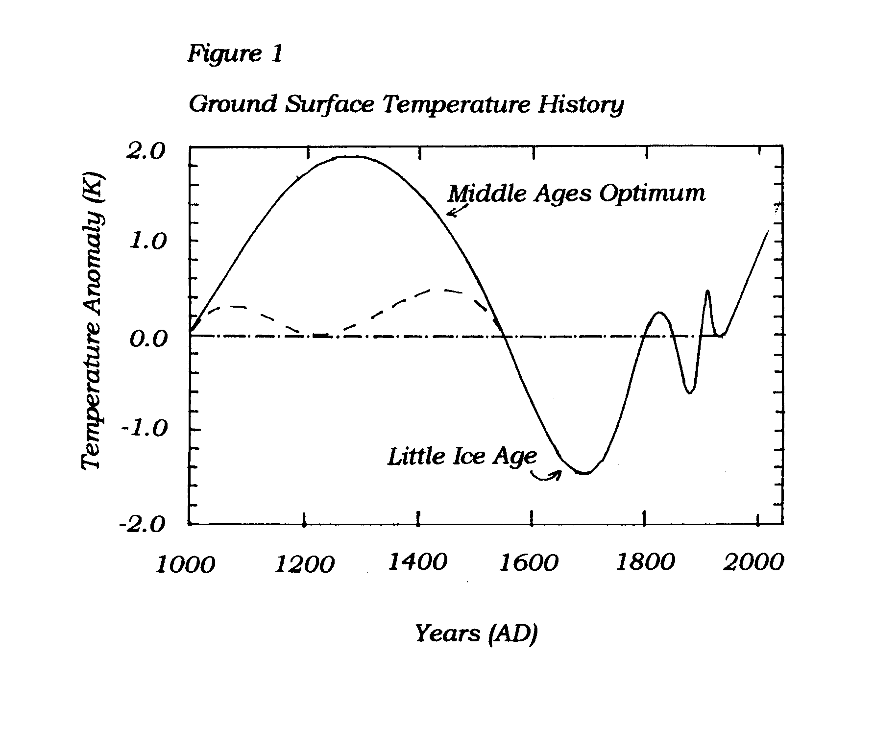
The penalty for misfit to data helps insure that whatever surface temperature history results from the analysis actually explains the observed borehole temperature. However, a common problem with obtaining the history of surface temperature from borehole temperatures is that heat conduction destroys information regarding long past temperature quite completely, and, therefore, many different different temperature histories explain the borehole data equally well. Quite a few of these histories oscillate in temperature wildly--far more, in fact, than the curve labelled "1" in Figure 1. By including a penalty for deviating from the initial model the objective function drives the final solution toward some unique result, and, if the initial model is smooth, the solution is also smooth.
Values in the matrices Cm and Cd provide an optimum balance between fitting the data (d) and adhering to an a priori model (mo). The matrix Cm deals with quantities in the a priori model; most specifically the initial estimate of ground surface temperature (GST) history while Cd deals with uncertainty in the temperature observations. Specifying small values for elements of these matrices implies that a person has great faith in the validity of the a priori model or the data. This is called a tight constraint. Specifying large values for these elements provides a loose constraint.
A presumption of the model is that there is a long-term steady state GST that may or may not equal the present day surface temperature, and a steady background thermal gradient which has to be removed before analysis. These are available from the data and the inverse method. The authors use loose constraints on these parameters, however; amounting to 100K and 500mW/m2, respectively. These are such loose constraints that they allow a background heat flow directed into the earth instead of out of it.
Constraining how far the final GST may stray from the initial temperature history also helps prevent an oscillating solution. The authors suggest a constraint that tightens more on older GST than on recent GST. Specifically, they allow recent GST history to stray about 4 times more from the initial model than they allow variation near 1000 years ago.
The tightening of constraint on GST implies that the authors have more faith in their initial ancient GST than they do in the recent GST. Certainly this is not consistent with the way borehole temperature behaves.

Three hypothetical GST histories. The dashed history shows no significant temperature variation until about 1600AD, exhibits a substantial cold period from then until 1800AD, vacillates over a few decades, and finally increases until the present time. By comparison, the dashed and dotted line is constant until approximately 1900AD and then begins the century-long temperature increase that we call "global-warming."
Some of results of this first study are unexpected. For example, a figure in the original paper shows the analysis of actual borehole temperatures. The GST derived from these diverges from one borehole to another in the recent past, but converges toward a zero value near 1000 years ago. Certainly this is unexpected. The physics of the problem suggests that the results would diverge most near 1000 years ago.
Similar behavior occurs in the numerical simulations the authors used to illustrate how loose constraints on thermal conductivity of the soil at a borehole can suppress noise and oscillations. Random noise added to the simulations had its largest effect on GST in the time period 1600-1700 AD when constraints on conductivity were tight and 1800-1850 AD when the constraints were loose.
The inverse method of this study suppresses large variations in GST for the most ancient time periods of an analysis in three ways.
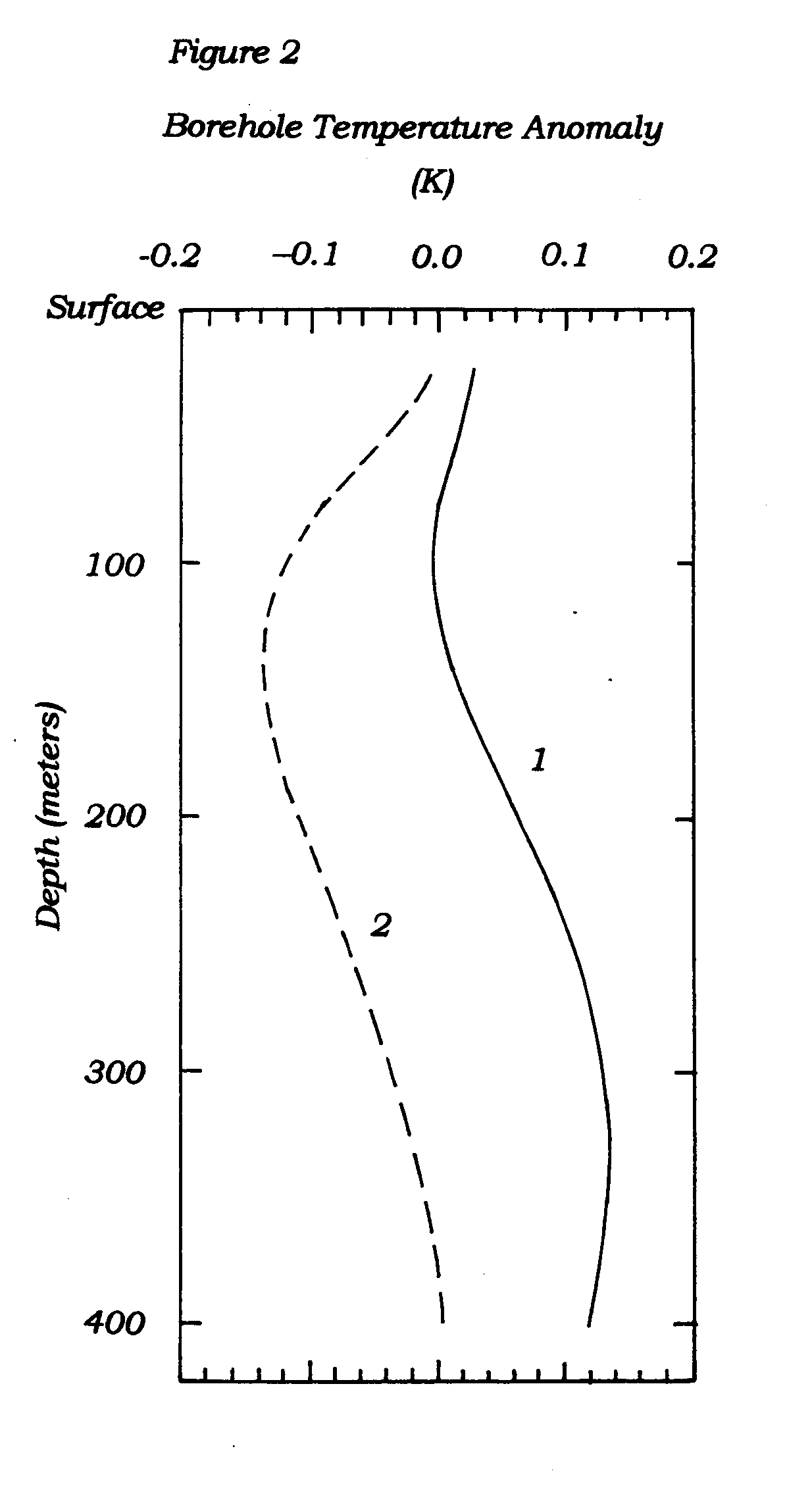
As an example of the third point consider the figure below. The curve labelled "2" shows the difference between the dashed and dotted curves of GST in Figure 1 at depths between surface and 400m. The beginning of the little ice age is not well resolved in this T-Z curve. In fact, it is nearly a linear increase of temperature with depth. With a small amount of added measurement noise, the inverse method would remove this linear increase along with the background temperature field, leaving only the recent climb out of the little ice age for analysis. The so-called steady state GST would equal the temperature appropriate to the little ice age, and the only GST change remaining is an increase beginning about 1800AD.

No invalid argument is implied in Study #1. However, in a subsequent study the same authors use this inverse method to examine the following problem. Divide the past 500 years into century long segments. Analyze a set of borehole temperatures to determine what GST change occured in each century.
The approach to the problem involves the following three steps, which taken together form a circular argument.
The authors interpret the zeroed GST as being characteristic of climate rather than being characteristic of assumptions and method. The conclusion may turn out to be perfectly correct for unrelated reasons, but the argument certainly appears circular and therefore invalid.
In the Principia Issac Newton presented examples of his mechanical system of the world. These examples acted as much to show the power of his system as they did to illustrate its uses. Through many editions of the text Newton worked with his editor to revise applications and maintain conformance with experimental findings. One body of experimental findings involved the speed of sound in air.
Newton understood very well the mechanical principles involved in sound propagation, but the specific details eluded him because of an incomplete understanding of heat transfer in a fast process. As a result Newton used the value of isothermal compressibility of air rather than isentropic compressibility, which left his estimates of sound speed wrong by 20% or so. However, to maintain the illusion that all was right with his mechanical system he engaged in a pattern of fudging the theory with ingenious, but unfounded and indefensible "corrections" to his calculations. Newton always knew what value for the speed of sound he needed to reproduce, which allowed him to fudge exact correction factors. This was circular reasoning, perhaps even outright dishonesty. Through the circular reasoning Newton managed to justify mechanical corrections that were non-existent. A well made circular argument can prove nearly anything.